Beyond one GPU: engineering distributed LLM inference

Video and frame credit: IBM Technology on YouTube ↗, presented by Grace Ableidinger. Watch the original: How AI Models Scale Beyond a Single GPU Across LLM Workloads ↗. The extracted frames are from that video; the additional diagrams, calculations, and implementation examples are Root18D’s independent commentary.

An enterprise assistant works in a demo, then stalls when fifty people paste long documents into it at the same time. The model has not become less capable. Its serving system has run out of a resource the demo never tested: space for active conversations, bandwidth between accelerators, or time inside the scheduler.

Buying more GPUs is an incomplete response. Four independent copies, four tensor shards, and four pipeline stages are three different systems. They move different data, fail differently, and produce different latency under the same traffic.

IBM Technology’s How AI Models Scale Beyond a Single GPU Across LLM Workloads ↗, presented by Grace Ableidinger, offers a useful visual introduction. Two selected frames anchor this field note. The capacity calculations, deployment example, control protocol, and calculator below are an independent engineering extension—not a claim that this cluster has been deployed or benchmarked.

This builds on Serving the token ↗: the question here is how to place the work across devices while preserving a useful service contract.

Define the service before choosing the topology

Consider a proposed document assistant with prompts up to 6,144 tokens and outputs capped at 2,048. Its initial acceptance targets are p95 time to first token below 1.5 seconds and p95 inter-token latency below 80 milliseconds, at a specified offered request rate. These are design targets, not measured results. Longer documents belong to a separately tested workload class.

A request succeeds only if it completes, meets the latency contract, and passes the application’s quality checks. Define operational goodput as completed requests meeting the serving SLO per second, then report quality acceptance separately. A server that generates tokens quickly but makes most users wait in a queue has not met the product requirement. DistServe ↗ frames disaggregated serving around goodput under first-token and per-token constraints.

Measure the entire path:

TTFT = gateway + queue + prefill + KV handoff + first decode step
E2E  = TTFT + subsequent decode time + stream delivery overhead

The handoff term is zero for a colocated engine. Each additional stage must earn its cost against this baseline.

Fit the live workload, not just the checkpoint

For dense BF16 weights, a first approximation is two bytes per parameter. An illustrative 72.7-billion-parameter model therefore requires 145.4 GB, or about 135.41 GiB, before activations, communication buffers, CUDA graphs, and KV cache. GB and GiB are different units; converting between them matters when a deployment is close to its memory limit.

For ordinary full-attention grouped-query attention, the logical cache size is:

KV bytes = 2 × layers × KV heads × head dimension
             × sum(active sequence lengths) × cache bytes per element

The leading two accounts for keys and values. Use KV heads, not query heads. Grouped-query attention ↗ shares key/value heads across groups of query heads. The public Qwen2.5-72B configuration ↗ supplies a concrete geometry: 80 layers, 64 query heads, eight KV heads, and hidden size 8,192, giving a head dimension of 128.

At 8,192 total tokens and two-byte cache elements, one sequence needs 2.5 GiB of logical KV state. With four-way tensor parallelism and evenly sharded KV heads, that is 0.625 GiB per GPU. Assuming 80 GiB physical memory, a 90% engine budget, and an additional 8 GiB runtime reserve per GPU:

Weights per GPU       = 135.41 / 4                  ≈ 33.85 GiB
Available KV per GPU  = 80 × 0.90 − 33.85 − 8        ≈ 30.15 GiB
Memory-only ceiling   = floor(30.15 / 0.625)        = 48 sequences

Forty-eight is not a recommended concurrency setting. This approximation assumes balanced weight placement and ignores cache-block rounding, uneven tensor placement, and transient peaks beyond the chosen reserve. The slowest or fullest rank governs the replica. At 32,768 tokens the same arithmetic falls to twelve sequences, without changing the model weights.

Run the downloadable calculator with Node.js; it needs no packages or GPU:

node inference-capacity.mjs
node inference-capacity.mjs '{"tokens":32768,"bandwidthGBs":12.5}'

It deliberately stops dividing KV memory when TP exceeds the number of KV heads; head replication can prevent further cache savings. It rejects unsupported fractional sharding and uneven pipeline splits. It is not a universal estimator for sliding-window attention, latent attention, hybrid state-space models, quantized metadata, or speculative decoding.

PagedAttention ↗ addresses another problem: managing cache blocks without requiring one large contiguous allocation per sequence. Better allocation reduces waste. It does not remove the bytes required by active tokens.

Choose what crosses the wire

Data parallelism adds complete serving replicas. A replica can itself span several GPUs. Requests are independent across replicas during ordinary inference; there is no training-style gradient synchronization. The router still needs health, queue, and cache information. Replication solves excess demand only after one complete replica fits and performs acceptably.

Pipeline parallelism assigns different layers to different stages. Intermediate activations move between stages. For a simple forward pipeline with P equal-duration stages and M independent microbatches, idealized utilization is approximately M / (M + P − 1). With four stages and one microbatch, that is 25%; with sixteen it is about 84%. Real autoregressive inference has dependencies between successive tokens and dynamic batches, so this is a bubble illustration, not a throughput predictor. GPipe ↗ develops layer partitioning and microbatch scheduling for training; inference needs its own scheduler measurements.

Tensor parallelism partitions the matrices inside a layer. A simplified feed-forward block can use column partitions for its first matrix and row partitions for its second:

H_i = activation(X × W_up_i)
Y_i = H_i × W_down_i
Y   = sum_i(Y_i)

The final sum requires communication. Real transformer implementations also distribute attention and may use different collective patterns. Megatron-LM ↗ explains complementary matrix partitions that keep some operations local. NCCL’s collective definitions ↗ distinguish all-reduce, all-gather, reduce-scatter, and all-to-all; they are not interchangeable costs.

A useful analytical approximation for a ring all-reduce of S bytes across N ranks is 2(N−1)α + 2(N−1)S/(Nβ), where α is per-hop latency and β effective bandwidth. The actual library may choose another algorithm. The formula explains why adding ranks can reduce local computation while increasing communication time. Benchmark message sizes from the intended batch shapes, not just peak network throughput.

The diagram illustrates two replicas, each using two four-GPU pipeline stages: sixteen GPUs total. It is an expansion option, not the starting footprint. vLLM’s distributed-serving guide ↗ supports combining TP and PP. Start by keeping frequent tensor collectives on the strongest interconnect and measuring whether cross-node layer partitioning meets the latency target. Physical placement must match logical ranks; eight available GPUs are not necessarily eight well-connected GPUs.

MoE changes placement, not the definition of free capacity

With mixture-of-experts models, active parameters determine only part of the per-token compute cost. All resident experts still consume memory. A learned router selects experts for each token; experts should not be assumed to map neatly to human labels such as “code” or “punctuation.” Selection patterns and specialization are empirical properties of the model.

Expert parallelism distributes expert weights and dispatches token activations to their owners. The dangerous case is skew: one expert rank becomes overloaded while fleet-average utilization looks healthy. Instrument token counts per expert, maximum-to-mean rank load, dispatch time, and combine time.

In the documented vLLM expert-parallel deployment ↗, enabling expert parallelism changes how MoE layers use the participating TP and DP ranks. EP size is derived from those groups; multiplying DP × TP × PP × EP blindly would double-count hardware. Validate the exact model, backend, and release combination before choosing that topology. The dense-model calculator above does not size an MoE deployment.

Separate prefill and decode only when the handoff pays

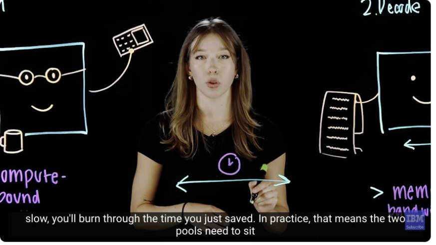
Prefill commonly exposes large matrix operations; small-batch decode often spends much of its time moving weights and cache data. Neither phase is permanently compute-bound or bandwidth-bound. Batch size, context length, quantization, and attention implementation can move the bottleneck.

The proposed split creates separate prefill and decode pools so each can use an appropriate scheduler and hardware shape. It also creates a distributed-state boundary. A full 8,192-token cache from the worked example is 2.5 GiB, or approximately 2.684 GB. At a measured aggregate 25 GB/s, its wire-time estimate is 107.4 ms; add an assumed 5 ms control overhead for approximately 112.4 ms. At 12.5 GB/s the estimate becomes 219.7 ms. Neither number includes queueing, contention, conversion, or additional replicated bytes.

A full cache is not always transferred. Prefix reuse, partial transfer, compression, and different connectors can change the volume. The calculator intentionally models an uncached full handoff so the assumption is visible.

The decision rule is workload-specific: saved interference and scheduling delay must exceed transfer, coordination, and any extra queueing delay while preserving the same quality and resource budget. vLLM’s disaggregated-prefill documentation ↗ labels the feature experimental and explicitly cautions against assuming a throughput improvement. Use it as a latency-isolation experiment. Start with continuous batching and chunked prefill before paying for another pool and transfer protocol.

Build a baseline that can actually be measured

The initial implementation is one four-GPU node with a dense model and colocated prefill/decode. Use a Linux CUDA environment with compatible drivers and a validated vLLM release. Record the container digest, model commit, tokenizer revision, GPU inventory, topology, and configuration with every benchmark. Download an approved immutable model snapshot to the path below before starting the service.

# Run on the GPU host, after installing the validated vLLM build.
# The model directory must contain the pinned weights and tokenizer.
nvidia-smi topo -m

vllm serve /models/qwen2.5-72b-instruct \
  --served-model-name document-assistant \
  --tensor-parallel-size 4 \
  --pipeline-parallel-size 1 \
  --dtype bfloat16 \
  --max-model-len 8192 \
  --gpu-memory-utilization 0.90 \
  --max-num-seqs 16 \
  --enable-chunked-prefill \
  --host 127.0.0.1 --port 8000

Sixteen concurrent sequences is a conservative experiment setting below the calculated memory ceiling, not a proven optimum. Startup profiling remains authoritative. If buffers or graphs exceed the assumed reserve, reduce the budget or sequence limit. Binding to loopback keeps this baseline reachable only locally; a production gateway would add authenticated access, tenant quotas, deadlines, and private service networking.

The public vLLM server argument reference ↗ defines these controls. Pin the version you validate rather than letting a mutable image change engine behavior between measurements.

For the 6,144-input / 2,048-output shape, run a bounded synthetic load test on that host:

vllm bench serve \
  --backend openai \
  --base-url http://127.0.0.1:8000 \
  --endpoint /v1/completions \
  --model document-assistant \
  --tokenizer /models/qwen2.5-72b-instruct \
  --dataset-name random \
  --random-input-len 6144 --random-output-len 2048 \
  --num-prompts 100 --request-rate 1 \
  --percentile-metrics ttft,tpot,itl,e2el \
  --metric-percentiles 50,95,99 \
  --goodput ttft:1500 tpot:80 \
  --save-result

The benchmark’s tpot condition is request-average time per output token; it does not replace the separate p95 inter-token-gap target. Inspect ITL percentiles as well. The benchmark CLI documentation ↗ defines these metrics and units. Synthetic token traffic tests serving mechanics, not answer quality. Replay representative, sanitized document tasks separately and score their outputs.

Admission control is a resource reservation

The gateway should tokenize the complete rendered prompt, including system instructions and tool schema. Reject requests exceeding the model context limit before they occupy GPU work. For accepted requests, reserve blocks for prompt length plus the permitted generation budget, or enforce a carefully measured growth policy.

A simple controller has a precise invariant:

For every rank in the chosen replica:
  reserved_KV_bytes + new_request_reservation <= safe_KV_budget

Within one atomic reservation transaction:
  verify replica health and exact model revision
  verify tenant quota and queue deadline
  reserve capacity on all participating ranks, or reserve none
  issue a lease with request ID, attempt ID, and expiry

A memory estimate alone is not this controller. Concurrent gateway workers must not read the same free capacity and both admit work against it. Use an authoritative scheduler or atomic reservation service. Release leases on completion and cancellation; reconcile expired leases with worker state before reuse. Sequence limits in the engine provide a second boundary, not a substitute for tenant fairness.

Cache-aware routing should use a bounded benefit: prefer a compatible warm prefix only when it saves more prefill work than the extra queue delay costs. Scope cache identity by model revision, adapter, tokenizer, template, exact token prefix, and the applicable tenant isolation boundary. A cache hit must never justify routing to an incompatible model revision.

Treat failures as part of the protocol

For a future disaggregated implementation, reserve decode capacity before generating transferable state. A transfer descriptor should identify request and attempt, model and adapter revisions, tokenizer, cache dtype/layout, token count, rank mapping, block IDs, byte count, integrity checks, and lease expiry. Decode acknowledges validation before prefill releases ownership.

If transfer fails before any output reaches the client, allow a bounded retry or recomputation on a healthy compatible replica, subject to the original deadline. If output has started, do not silently restart and concatenate a second stochastic answer. Return an explicit partial-stream failure with a request ID. Application-level tool side effects need their own idempotency contract; a generation retry does not undo an already executed tool.

Kill a worker during load testing. Verify that routing stops admitting to the affected replica, reservations clear safely, healthy replicas do not receive an unbounded retry storm, and clients see the defined failure behavior. A system can meet latency targets during steady state and still be unusable during routine maintenance.

Promote evidence, not GPU utilization

Trace gateway admission, queueing, prefill, cache transfer, decode, and stream completion under one request/attempt lineage. Record token counts, model revision, TP/PP configuration, topology, cache allocations, retries, and cancellation latency. Keep raw prompts out of routine telemetry. Request IDs belong in traces; putting one in every metrics label creates uncontrolled cardinality.

Compare the four-GPU baseline against a second replica, a changed TP layout, and eventually a disaggregated configuration under the same arrival pattern. Include short chat, long documents, burst traffic, cold prefixes, and worker loss. Sweep offered load gradually until the SLO fails, rather than presenting one favorable concurrency point.

For each experiment, report p50/p95/p99 TTFT and ITL, errors, completed SLO-compliant requests per second, quality acceptance, and total provisioned cost per accepted task. Count idle reservation, warm standby, CPU, networking, and failed attempts in the numerator. More GPUs are valuable only when the extra capacity improves a customer outcome at an acceptable cost.

The practical first release is deliberately small: one pinned model, one topology, a measured traffic envelope, enforced admission, observable failures, and a repeatable benchmark record. Add another dimension of parallelism when that record identifies the constraint it will remove.